General Purpose Coarse-Grained Force Field

Introduction

In this tutorial, we will discuss how to convert a Martini 3 [1] system into a titratable Martini [2] one and perform constant pH simulations.

Please note that this tutorial makes use of Python 3 and several of its external modules. So make sure that you have Python 3 installed in your system together with the following external modules (pip install module_name): numpy, pandas, matplotlib, MDAnalysis, pymbar, tdqm.

To get started, download the archive (titratable_martini_tutorial_files.zip), which contains necessary files for this tutorial. Extract the contents of the ZIP file in your working directory and you are ready to begin! Additionally, you can download the worked version of this tutorial to either get some hints or to compare your results.

Note that these MD simulations might take several hours depending on your computational resources. You can always reduce the number of pH data points and/or shorten the simulation times to fasten the process if you have limited resources: The fitted pKa values will lose accuracy and precision but you will still get acquainted with the methodology. Alternatively, you can use the trajectory files from the worked example instead of running the simulations.

1 Acid titration

In this example, we will study the titration of acetic acid. Go to the directory 1_acid_titration. As the starting point, we have a standard Martini 3 system with 16 acetic acid molecules (P2 beads) and 1936 water beads.

1.1 Converting the system to Titratable Martini

The first step is to convert your existing standard Martini 3 coordinate file (standard.gro) into a titratable one by running the script 1_convert_gro_file.sh. The script contains:

Here, the -f and -o flags set the input and out files, respectively. -sel selects the bead that will be converted to the titratable version. Any selection command from MDAnalysis can be used, but we will stick with the name command, which selects based on the atom/bead name. -bead specifies the type of that bead (water, acid, base, acid-deprot, base-deprot). The script is called here twice since we have two type of titratable beads in the system: In the first step acetic acid (P2) beads are converted, which correspond to acid beads; in the second step, water beads (WN) are converted, which clearly have the type water. convert_gro_to_titratable.py script adds the necessary dummy particles and H⁺ ions to each titratable bead type as described in the article [2]. The titratable version of the coordinate file start.gro can now be found in the same directory.

The next next step is to create a topology file (system.top, see below) corresponding to the titratable system. Here, the first line (#define pH<value>) is where the pH of the system is defined. <value> will be replaced by the actual pH value that we are interested in. For example, for a pH of 3, this line would read: #define pH3.0. Acceptable pH values range from 3 to 8 with increments of 0.25. In the next two lines, we link to the titratable Martini force field (martini.itp) and the already parametrized titratable molecules (molecules.itp). Finally, in the [molecules] block, we specify the molecules that are present in the system. Here, we still have 16 acetic acid (PPA) molecules, 1936 water beads (WNA) just as the standard system. Additionally, we now have 1952 H⁺ ions, one for each titratable site (16+1936).

1.2 Titration

Now that we have both the coordinate (start.gro) and the topology (system.top) files, we are ready to begin the titration! This will be done by running the script 2_titrate.sh. This script simply changes the pH value in the system.top file and starts the necessary MD runs. In this tutorial, we will titrate from pH=3.0 to 8.0 with increments of 0.5.

At each pH, we will perform energy minimization, equilibrium and production runs. The corresponding run parameters (.mdp) are given in the directory mdp_files. Note that these parameters are specifically for the titratable Martini simulations and are different than the standard Martini 3 run parameters (see the paper for the discussion [2]).

1.3 Analysis

After the simulations have finished, we can proceed with the analysis. This will be done by running the script 3_analyze.sh. At each pH, this script calls degree_of_deprot.py, which computes the degree of deprotonation of the system (see the paper for the methodology [2]). Here, with -f, -s and -o flags the trajectory, topology and output file names, respectively, are given. The flag -b sets the starting simulation time (picoseconds) for analysis. The flags -ref and -sel again uses the MDAnalysis selection commands for the reference and the titratable bead, respectively. In this case, our reference is water (WN) and the selection is the titratable and the only bead of acetic acid (P2).

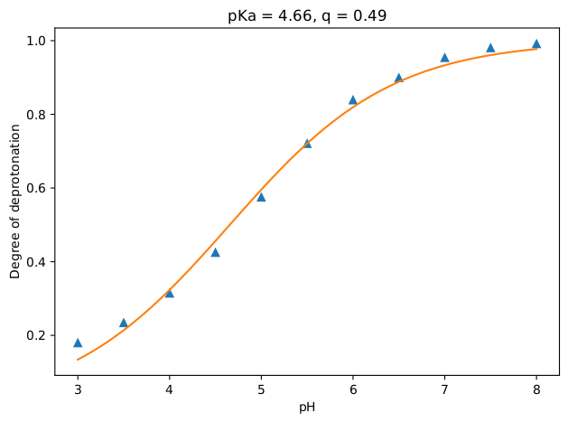
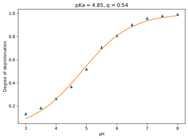
The results, which are the degrees of deprotonation at each pH, are written to the text file results.txt. Additionally, a plot is generated (results.pdf ) containing these data points and the computed pKa and q value by fitting the results to the following equation:

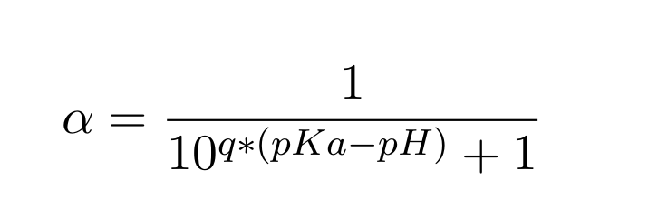(1)

There you have it! If all went well, you should have a plot that looks like the figure below. As expected, the acetic acid becomes more and more protonated as the pH value is decreased.

2 Base titration

In this example, we will study the titration of aniline. Go to the directory 2_base_titration. As the starting point, we have a standard Martini 3 system with a single aniline molecule and 2021 water beads. Since this exercise is mostly similar to the acid titration, we will only go over the main differences.

2.1 Converting the system to Titratable Martini

The main difference when converting the coordinate file is that in this case the titratable bead is a base instead of an acid. This again is specified with the -bead flag.

Next difference is the [molecules] block of the topology file (system.top). We now have a single aniline molecule (ANIL) and 2021 water beads (WNA). These water beads also contain H⁺ ions. Note that unlike the acid bead, the base bead does not contain an H⁺ ion. Consequently, the [molecules] block looks like:

2.2 Titration

This part goes exactly the same as previous exercise.

2.3 Analysis

This part also goes exactly the same as previous exercise, except the results of course. If all went well, you should have ended up with a titration curve that looks like the figure below. As expected, aniline becomes more and more protonated as the pH value is decreased.

3 Environment dependent pKa shifts

Capturing changes in the apparent pKa due to interactions with the environment is one of the most important aspects of any constant pH simulation methodology. In this example, we will study the environment dependent pKa shift of the G5 dendrimer poly(propylene imine) (PPI). Go to the directory 3_environment_dependent_pka_shifts. As the starting point, we have a standard Martini 3 system with a single G5 PPI dendrimer and 1936 water beads. Again, the parts that are similar to the previous exercises will not be explained in detail.

3.1 Converting the system to Titratable Martini

In this case, the G5 PPI dendrimer contains 126 titratable base sites. As all these bead names starts with N, we use an asterisk for selection (-sel "name N*") for the generation of the titratabe version of the coordinate file. For the topology file, as in the previous example, only the water beads contain an H⁺ ion. Consequently, the [molecules] block looks like:

3.2 Titration

This part goes exactly the same as previous exercise.

3.3 Analysis

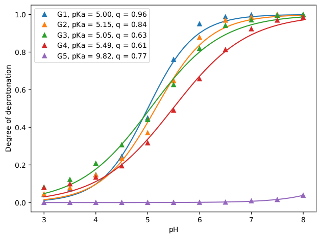
For this exercise, we can analyze using the 3_analyze.sh script the degree of deprotonation separately for each generation of the dendrimer to see the effect of the environment on the degree of (de)protonation. Here, G1 is the innermost generation and G5 is the outermost. The separate analysis is done by specifying for each generation all other titratable sites as the reference. For example for calculating the degree of deprotonation of G1, we select the G1 beads ("-name NG1") with the -sel flag and the rest ("-name WN NG2 NG3 NG4 NG5") as the reference with the -ref flag. You can see the results of this analysis below: At high pH values (~7-8), only the outermost generation (G5) is protonated, as the pH is lowered (5-6), the inner generations starts becoming partially protonated and at even lower pH values (3-4), all titratable sites are almost fully protonated. This is also apparent from the fitted pKa values: G5 has the highest pKa value (9.8), followed by G4 (5.5), then, the three inner generations have similar low pKa values (~5).

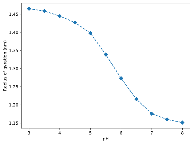
The radius of gyration will also be computed as a function of pH with the same analysis script and its results are shown in the figure below. It can be seen that the dendrimer expands with the decrease of pH. This correlates well with the increased amount of protonated residues.

References

[1] P. C. T. Souza, R. Alessandri, J. Barnoud, S. Thallmair, I. Faustino, F. Grünewald, I. Patmanidis, H. Abdizadeh, B. M. H. Bruininks, T. A. Wassenaar, P. C. Kroon, J. Melcr, V. Nieto, V. Corradi, H. M. Khan, J. Domański, M. Javanainen, H. Martinez-Seara, N. Reuter, R. B. Best, I. Vattulainen, L. Monticelli, X. Periole, D. P. Tieleman, A. H. de Vries, S. J. Marrink, Nat. Methods 2021, 18, 382–388.
[2] F. Grünewald, P. C. T. Souza, H. Abdizadeh, J. Barnoud, A. H. de Vries, S. J. Marrink, J. Chem. Phys. 2020, 153, 024118.