General Purpose Coarse-Grained Force Field

1: Lipid bilayers I — Self-assembly

Details

Last Updated: Wednesday, 01 September 2021 00:19

A PDF version of this tutorial is available here.

In case of issues, please contact This email address is being protected from spambots. You need JavaScript enabled to view it. or This email address is being protected from spambots. You need JavaScript enabled to view it.

Introduction

The Martini coarse-grained (CG) model was originally developed for lipids^[1,2]. The underlying philosophy of Martini is to build an extendable CG model based on simple modular building blocks and to use only few parameters and standard interaction potentials to maximize applicability and transferability. Martini 3 greatly expanded the number of possible interactions, but retains this building-block approach^[3]. Due to the modularity of Martini, a large set of different lipid types has been parameterized. Their parameters are available with the Martini 3 Release archive. In this tutorial, you will learn how to set up lipid-water system simulations with lipids from this collection, with a focus on bilayers. You will also study a number of standard bilayer properties. 

These tutorials assume a basic understanding of the Linux operating system and the gromacs molecular dynamics (MD) simulation package. Excellent gromacs tutorials are available at: http://www.mdtutorials.com/gmx/. 

The aim of the tutorial is to create and study properties of CG Martini models of lipid bilayer membranes. First, we will attempt to spontaneously self-assemble a DPPC bilayer and check various properties that characterize lipid bilayers, such as the area per lipid, bilayer thickness, order parameters, and diffusion. Next, we will change the nature of the lipid head groups and tails, and study how that influences the properties. In the Lipid Bilayers II tutorial you will move on to creating more complex multicomponent bilayers.

You can download all the files, including worked examples of this tutorial (GROMACS version 2021): LipidBilayers_Part1_Worked.tar.gz. This is a rather large archive. A smaller set that expects you to do more yourself is recommended and is named: LipidBilayers_Part1.tar.gz. Unpack one of the lipidome-tutorial.tgz archives (NOTE: both expand to a directory called bilayer-lipidome-tutorial), and enter the bilayer-lipidome-tutorial directory:

$ tar -xzvf LipidBilayers_Part1.tar.gz

$ cd bilayer-lipidome-tutorial 

Bilayer self-assembly

We will begin with self-assembling a dipalmitoyl-phosphatidylcholine (DPPC) bilayer from a random configuration of lipids and water in the simulation box. Enter the spontaneous-assembly/initial_assembly subdirectory. The first step is to create a simulation box containing a random configuration of 128 DPPC lipids. This can be done by starting from a file containing a single DPPC molecule, which you can get from the Martini lipidome, under the entry for DPPC. Download the DPPC-em.gro file (but not any.itp file from there, as those are specific for Martini 2):

$ wget http://cgmartini.nl/images/parameters/lipids/PC/DPPC/DPPC-em.gro

Note the remark on the lipidome’s DPPC page, which will be relevant later on, that the model “corresponds to atomistic C16:0 dipalmitoyl (DPPC) - C18:0 distearoyl (DSPC) tails”. This reflects that, in Martini, the 4-to-1 mapping in acyl tails limits the resolution and the same model represents in this case a C-16 tail (palmitoyl) and a C-18 tail (stearoyl, hence DSPC).

Also note that you can download coordinate files for many Martini lipids from the website. For the time being these structures are mostly for Martini 2 lipids, but structurally the difference doesn’t matter in the cases, like DPPC, where the Martini 3 lipid has the same mapping and number of beads. Finally, for cases when you have a lipid topology but not its structure, see the Lipid Bilayers II tutorial on using the insane script, or look into the molmaker.py script for generating structures directly from topologies.

The gromacs tool insert-molecules can take the DPPC-em.gro this single-molecule conformation and attempt to place it in a simulation box multiple times at a random position and random orientation, each time checking that there are no overlaps between the consecutively placed molecules. For help on any gromacs tool, you can add the -h flag.

$ cd spontaneous-assembly/initial_assembly

$ gmx insert-molecules -ci DPPC-em.gro -box 7.5 7.5 7.5 -nmol 128 -radius 0.21 -try 500 -o 128_noW.gro 

The value of the flag -radius (default van der Waals radii) has to be increased from its default atomistic length (0.105 nm) to a value reflecting the size of Martini CG beads. The output filename is arbitrary but we choose one ending in _noW to indicate ‘no Water’.

Using the gromacs tool solvate, add 6 CG waters per lipid (note that this corresponds to 24 all-atom waters per lipid, 768 in total). gmx solvate needs to have the structure of an equilibrated water box to use as a template to fill the empty space in 128_noW.gro. The website has one (water.gro) available for you under the Example applications -> Solvent systems section; download it:

$ wget http://cgmartini.nl/images/applications/water/water.gro

You can now run solvate:

$ gmx solvate -cp 128_noW.gro -cs water.gro -o waterbox.gro -maxsol 768 -radius 0.21

Also here, the value of the flag -radius is used to reflect the size of Martini CG beads. A new file, waterbox.gro is produced containing the 128 lipids and added water beads.

Now you will perform an energy minimization of the solvated system, to get rid of high forces between beads that may have been placed quite close to each other. The settings file minimization.mdp is provided for you, but you will need the topology for water and for the DPPC lipid, and to organize them as a .top file. From the website’s Force field parameters -> Particle definitions section you can get the zip file for the Martini 3 release, which contains the relevant topologies:

$ wget http://cgmartini.nl/images/martini_v300.zip

$ unzip martini_v300.zip

Note that the Martini 3 release is organized into several .itp files, each with the definitions for a class of molecules. For this tutorial you won’t need all of the Martini 3 .itps, only the one where water is defined (hint: it’s a ‘solvent’) and the one where DPPC is defined (hint: it’s a ‘phospholipid’). There is a third .itp you will need, and that is the one with all the Martini 3 particle definitions (hint: it’s martini_v3.0.0.itp). The needed .itps should be placed in the tutorial directory.

To create the .top file (we’ll call it dppc.top) that describes the system topology to GROMACS, you can follow the template below. Semi-colons indicate comments, which are ignored, but hashtags aren’t: they’re preprocessing directives. Namely, it is the #include directive that allows us to bring into the .top the particle/molecule information in the .itps. Use your editor of choice (gedit/vi/other) to create a file dppc.top, copy the template into it and complete the ‘…’ fields (hint: to figure out how many waters to set, look at the output of gmx solvate to see how many W beads were added; the maximum number is 768, as specified with the -maxsol option).

You are now ready to perform an energy minimization.

$ gmx grompp -f minimization.mdp -c waterbox.gro -p dppc.top -o dppc-min-solvent.tpr 

$ gmx mdrun -s dppc-min-solvent.tpr -v -c minimized.gro

Now, you are ready to run the self-assembly MD simulation, by using the martini_md.mdp run settings file and the just-minimized minimized.gro. 30 ns, or 1.5 million simulation steps at 20 fs per step, should suffice.

$ gmx grompp -f martini_md.mdp -c minimized.gro -p dppc.top -o dppc-md.tpr

$ gmx mdrun -s dppc-md.tpr -v -x dppc-md.xtc -c dppc-md.gro

This might take approximately 10 minutes on a single CPU but by default gmx mdrun will use all available CPUs on your machine. The -v option shows an estimate of the time to completion, and it is interesting to observe how the generations of desktop computers have sped up this 30 ns simulation over the years. See gmx mdrun’s help (-h) for instructions on how to tune the numbers of parallel threads gmx mdrun uses. You may want to check the progress of the simulation to see whether the bilayer has already formed before the end of the simulation. You may do this most easily by starting the inbuilt gromacs viewer (you will need to open a new terminal and make sure you are in the directory where this simulation is running):

$ gmx view -f dppc-md.xtc -s dppc-md.tpr

or, alternatively, use VMD or pymol. Both VMD and pymol suffer from the fact that Martini bonds are usually not drawn because they are much longer than standard bonds and the default visualization is not very informative. For visualization with pymol this is solved most easily by converting the trajectory to .pdb format, explicitly writing out all bonds (select System or DPPC, depending on whether you want to visualize the entire system or only the lipids). The disadvantage is that very large files are produced in this conversion!

$ gmx trjconv -s dppc-md.tpr -f dppc-md.xtc -o dppc-md.pdb -pbc whole -conect

$ pymol dppc-md.pdb

For VMD, a plugin script cg_bonds-v5.tcl was written that takes the GROMACS topology file and adds the Martini bonds defined in the topology (this file is included in the directory for your convenience, but you would normally want to download it from the Tools -> Visualization section of the website, store it in a generally useful location and refer to it when needed). A useful preprocessing step for VMD visualization is to avoid molecules being split over the periodic boundary, because if they are, very long bonds will be drawn between them. A script do_vmd.sh has been prepared for you for visualization using VMD. You will probably need to make the script executable.

$ chmod +x do_vmd.sh

$ ./do_vmd.sh

The initial and final snapshots should look similar to Fig. 1, at least if the self-assembly resulted in a bilayer in the allotted time, which is not guaranteed. You may have noticed, however, that there is relatively little water, and some part of the initial solvated box is actually devoid of water. This helps to more or less guarantee a bilayer, but does make the simulation a little less realistic. You can test by solvating the lipids with more solvent. You can do this by changing the  -maxsol flag on the  gmx solvate command.

In the meantime, have a close look at the DPPC section of the phospholipid .itp file. The available bead types and their interactions are defined in martini_v3.0.0.itp and described in the 2021 Martini 3 paper^[3]. Understanding how these files work, will help you work with the Martini 3 model and define new molecules or refine existing models.

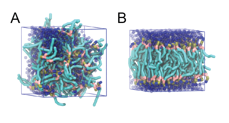
Figure 1 | DPPC bilayer formation. A) 64 randomly localized DPPC lipid molecules with water. B) After a 30 ns long simulation the DPPC lipids have aggregated together and formed a bilayer.

When the simulation has finished, check whether you got a bilayer. If yes, check if the formed membrane is normal to the z-axis (i.e., that the membrane is situated in the xy-plane). Have a look at the self-assembly process: can you recognize intermediate states, such as micelles, and do you see metastable structures such as a water pore (water spanning the membrane interior) and/or a lipid bridge (lipid tail(s) spanning the water layer)?

Bilayer equilibrium run and analysis

If your bilayer was formed in a plane other than the xy-plane, rotate the system so that it will (with gmx editconf). In case you did not get a bilayer at all, you can continue the tutorial with the pre-formed one from dspc-bilayer.gro. (Example files of the tutorial assume that this file is used.) From this point on, we will refer to the bilayer as a DSPC bilayer. As remarked earlier, in Martini, the 4-to-1 mapping of acyl tails limits the resolution and the same model represents in this case a C-16 tail (palmitoyl) and a C-18 tail (stearoyl, hence DSPC). The reason for referring to the lipid as DSPC is that later on, we will compare the simulated properties to experiment and we will compare different lipids all with the same number of beads, changing either the head group from PC to PE or changing the tail from stearoyl (C-18, fully saturated) to oleoyl (C-18, single cis double bond at C-9). 

The spontaneous assembly simulation was done using isotropic pressure coupling. The bilayer may have formed but is probably under tension because of the isotropic pressure coupling. Therefore, we first need to run a simulation in which the area of the bilayer can reach a proper equilibrium value. This requires that we use independent pressure coupling in the plane and perpendicular to the plane. Set up a simulation for another 30 ns at zero surface tension (switch to semi-isotropic pressure coupling; if the pressure is the same in the plane and perpendicular to the plane, the bilayer will be at zero surface tension) at a higher temperature of 341 K. This is above the experimental gel to liquid-crystalline transition temperature of DSPC (you will find how to change pressure coupling and temperature in the gromacs manual).

It is highly recommended that you make perform this simulation in a new directory, name it, for example equilibration. Copy the required files there, edit the .mdp file, and set the run going (the commands for this final step — involving gmx grompp and gmx mdrun — are not given explicitly).

$ mkdir ../equilibration

$ cp dppc-md.gro (or dspc-bilayer.gro) ../equilibration/.

$ cp martini_md.mdp ../equilibration/.

$ cp martini*.itp ../equilibration/.

$ cp dppc.top ../equilibration/.

$ cd ../equilibration

$ [gedit/vi] martini_md.mdp

Then prepare a .tpr file (gmx grompp etc) and run the simulation (gmx mdrun etc; i.e. similar instructions as for the spontaneous assembly run explained above). If you do not want to wait for this simulation to finish, skip ahead and use a trajectory provided in the fully worked tutorial archive. NOTE!! The commands below assume your production run is producing files with the prefix md. This need not be the case, so replace these entries with the appropriate name(s) for your simulations.

If you have difficulty in running the simulation you may want to use the 30 ns trajectory already present in the subdirectory spontaneous-assembly/equilibration/ of the worked example.

From the latter simulation, we can calculate properties such as:

• area per lipid

• bilayer thickness

• P₂ order parameters of the bonds

• lateral diffusion of the lipids

In general, for the analysis, you might want to discard the first few ns of your simulation as equilibration time. The area per lipid as a function of time should give you an indication of which part of the simulation you should definitely not include in the analysis. 

Area per lipid

To get the (projected) area per lipid, you can simply divide the area of your simulation box by half the number of lipids in your system. The box-sizes can be obtained by running the gromacs tool gmx energy (ask for Box-X and Box-Y, remember that gmx 'tool' -h brings up the help of any gromacs tool). To calculate the area per lipid as a function of time we’ll use a couple of python lines (though many alternative methods are possible). The gromacs tool analyze provides a convenient way to then calculate the average and error estimate in any series of measurements (use the option -ee for the error estimate, and make sure you feed gmx analyze a file with a .xvg extension). (Note that this calculation might not be strictly OK, because the self-assembled bilayer might be slightly asymmetric in terms of number of lipids per monolayer, i.e., the areas per lipid are different for the two monolayers. However, to a first approximation, we will ignore this here.)

$ gmx energy -f md.edr -o box-xy.xvg

     > 11 12 0 [press Enter]

Here, the second line is meant to show that you need to type the number(s) of the property/ies you want. In our version this is 11 for Box-X and 12 for Box-Y. After typing "Enter" the output file is produced. You can visualize it in xmgrace:

$ xmgrace -nxy box-xy.xvg

To obtain the area per lipid, you need to multiply the values of x and y at each timepoint, and divide by 64 (number of lipids per monolayer or leaflet). To do this start a python3 session in your command line and run the following lines:

import numpy as np

xy = np.loadtxt('box-xy.xvg', comments=('#','@'))

areas = xy[:,1] * xy[:,2] / 64

np.savetxt('area.xvg', np.column_stack((xy[:,0], areas)))

[ Exit the python interpreter by pressing Ctrl+D ]

This will create file area.xvg, which you can visualize with xmgrace:

$ xmgrace area.xvg

Next, get the averages and error estimates using the gromacs tool analyze. You can discard what you deem to be the relaxation time by using the flag  -b [initial time to ignore].  

$ gmx analyze -f area.xvg -ee

$ gmx analyze -f area.xvg -ee -b 15000

As an alternative you can use awk  to calculate the area per lipid. Then look at the statistics. 

$ awk '{if (substr($1,1,1) != "#" && substr($1,1,1) != "@") print $1, $2*$3/64}' < box-xy.xvg > area.xvg

$ gmx analyze -f area.xvg -ee -b 15000

Bilayer thickness

To get the bilayer thickness, use gmx density. You can get the density for a number of different functional groups in the lipid (e.g., phosphate and ammonium headgroup beads, carbon tail beads, etc) by feeding an appropriate index-file to gmx density (make one with gmx make_ndx; you can select, e.g., the phosphate beads by typing a P*; type q to exit , this leaves you with an index file named  index.ndx). You can obtain an estimate of the bilayer thickness from the distance between the headgroup peaks in the density profile.

$ gmx make_ndx -f md.gro

    > a P*

    > q

$ gmx density -f md.xtc -s md.tpr -b 15000 -n index.ndx -o p-density.xvg -xvg no

    > 4

$ xmgrace p-density.xvg 

A more appropriate way to compare to experiment is to calculate the electron density profile. The gmx density tool also provides this option. However, you need to supply the program with a data-file containing the number of electrons associated with each bead (option -ei electrons.dat). The format is described in the gromacs manual and not part of this tutorial.

Compare your results to those from small-angle neutron scattering experiments^[4]:

• thickness = 4.98 ± 0.15 nm

• area per lipid = 0.65 ± 0.05 nm²

Lateral diffusion

Before calculating the lateral diffusion, remove jumps over the box boundaries (gmx trjconv -pbc nojump). Then, calculate the lateral diffusion using gmx msd. Take care to remove the overall center of mass motion (-rmcomm), and to fit the line only to the linear regime of the mean-square-displacement curve (-beginfit and -endfit options of gmx msd). To get the lateral diffusion, choose the -lateral z option.

$ gmx trjconv -f md.xtc -s md.tpr -pbc nojump -o nojump.xtc

$ gmx msd -f nojump.xtc -s md.tpr -rmcomm -lateral z -b 15000

$ xmgrace msd.xvg

In comparing the diffusion coefficient obtained from a Martini simulation to a measured one, one can expect a faster diffusion at the CG level due to the smoothened free energy landscape (note, however, that the use of a defined conversion factor is no longer recommended, as it can vary significantly depending on the molecule in question). Also note that the tool averages over all lipids to produce the MSD curve. It is probably much better to analyze the motion of each lipid individually and remove center-of-mass motion per leaflet. This requires some scripting on your part and is not included in this tutorial.

Order parameters

Now, we will calculate the (second-rank) order parameter, which is defined as:

P₂ = 1/2 (3 cos²<θ> − 1),

where θ is the angle between the bond and the bilayer normal. P₂ = 1 means perfect alignment with the bilayer normal, P₂ = −0.5 anti-alignment, and P₂ = 0 random orientation.

A script to calculate these order parameters can be downloaded in the Tools -> Other tools section of the website (scroll down to the section on do_order, and download the script do-order-gmx5.py. There is also a version located in the directory scripts/). Copy the .xtc and .tpr files to an analysis subdirectory (the script expects them to be named traj.xtc and topol.tpr, respectively). The script do-order-gmx5.py will calculate P₂ for you. As it explains when you invoke it, it needs a number of arguments. You may need to or want to change some of the arguments. The command:

$ python do-order-gmx5.py md.xtc md.tpr 15000 30000 20 0 0 1 128 DPPC

Will, for example, read 15 to 30 ns from the trajectory md.xtc. The simulation has 128 DPPC lipids and the output is the P_2, calculated relative to the Z-axis, and average over results from every 20th equally-spaced snapshot in the trajectory. Results are available as output and in the files order.dat and S-profile.dat; the latter is a profile that can be compared to published profiles, e.g. in Ref.^[1] (remember, DSPC and DPPC share the same Martini representation!).

Advanced: additional analyses

Different scientific questions require different methods of analysis and no set of tools can span them all. There are various tools available in the gromacs package, see the gromacs manual. Most simulation groups, therefore, develop sets of customized scripts and programs many of which they make freely available, such as the Morphological Image Analysis and the 3D pressure field tools available here. Additionally a number of packages are available to for assistance with analysis and the development of customized tools, such as the python MDAnalysis package.

Changing lipid type

Lipids can be thought of as modular molecules. In this section, we investigate the effect of changes in the lipid tails and in the headgroups on the properties of lipid bilayers using the Martini model. We will i) introduce a double bond in the lipid tails, and ii) change the lipid headgroups from phosphatidylcholine (PC) to phosphatidylethanolamine (PE).

Unsaturated tails

To introduce a double bond in the tail, we will replace the DSPC lipids by DOPC. Set up a directory for the DOPC system. Enter that directory. Compare the Martini 3 topologies of these two lipids in the phospholipids .itp. You will see that the number of beads for these lipids is the same, and in the same headgroup-glycerol-tails order. You can therefore set up a DOPC bilayer quite simply from your DSPC result. Copy over the .top and .mdp file from the equilibration DSPC run. Copy the final frame of the DSPC run to serve as the starting frame of the DOPC run. Replace DPPC by DOPC in your .top and .mdp files, and gmx grompp will do the rest for you (you can ignore the ”atom name does not match” warnings of grompp); you do this by adding the -maxwarn option to the gmx grompp command, e.g. gmx grompp -maxwarn 3 allows a maximum of 3 warnings and will still produce a .tpr file). Execute the simulation, or, if you are impatient, use the trajectory provided for you as spontaneous-assembly/equilibration/dopc/dopc-ext.xtc. NOTE: if you take this shortcut, and because the lipids DSPC and DOPC have exactly the same number of beads, you can use the .tpr file from DSPC to analyze the dopc-ext.xtc file. 

Changing the headgroups

Similarly, starting again from the final snapshot of the DSPC simulation, you can easily change the head groups from PC to PE, yielding DPPE. Also for this system, run a 30 ns MD simulation, or, if you are impatient, use the trajectory provided for you as spontaneous-assembly/equilibration/dspe/dspe-ext.xtc. NOTE: as above, when taking this shortcut, and because the lipids DSPC and DPPE have exactly the same number of beads, you can use the .tpr file from DSPC to analyze the dspe-ext.xtc file.

Compare the above properties (area per lipid, thickness, order parameter, diffusion) between the three bilayers (DSPC, DOPC, DSPE). Do the observed changes match your expectations? Why/why not? Discuss.

Tools and scripts used in this tutorial

gromacs (http://www.gromacs.org/)

[1] Marrink, S. J., De Vries, A. H., and Mark, A. E. (2004) Coarse grained model for semiquantitative lipid simulations. J. Phys. Chem. B 108, 750–760. DOI:10.1021/jp036508g

[2] Marrink, S. J., Risselada, H. J., Yefimov, S., Tieleman, D. P., and De Vries, A. H. (2007) The MARTINI force field: coarse grained model for biomolecular simulations. J. Phys. Chem. B 111, 7812–7824. DOI:10.1021/jp071097f

[3] Souza, P. C. T., Alessandri, R., et al. (2021) Martini 3: a general purpose force field for coarse-grained molecular dynamics. Nat. Methods 18, 382–388. DOI: 10.1038/s41592-021-01098-3

[4] Balgavy, P., Dubnicková, M., Kucerka, N., Kiselev, M. A., Yaradaikin, S. P., and Uhrikova, D. (2001) Bilayer thickness and lipid interface area in unilamellar extruded 1,2-diacylphosphatidylcholine liposomes: a small-angle neutron scattering study. Biochim. Biophys. Acta 1512, 40–52. DOI:10.1016/S0005-2736(01)00298-X