


Martini tutorials: Free energy techniques
- Details
- Last Updated: Friday, 21 October 2022 11:00
Martini tutorials: Free energy techniques
If you just landed here, we recommend you follow the tutorial about lipid bilayers first.
Summary
Introduction
The aim of this set of practicals is to familiarize with free energy techniques using the Gromacs program suite and the coarse-grained (CG) force field Martini. You will learn how the necessary input files are structured, how to set up and run the simulations, and finally how to extract the required information from the simulations.
In particular, we will calculate the partition coefficient of a CG bead in water and hexadecane using free sampling, umbrella sampling and thermodynamic integration. These methodologies have a number of practical applications, e.g. to study free energies of solvation/hydration, free energies of binding of a small molecule (e.g. a drug molecule) to a receptor (e.g. a protein), and the free energy cost of point mutations.
All files needed for this part of the tutorial can be found in the FreeEnergyTechniques folder in FreeEnergyTechniques.zip. Each part of this tutorial has its own directory which itself contains a folder called files_DoItYourself. There you can find the necessary files to follow the tutorial. For the second and the third part (umbrella sampling and thermodynamic integration) we also provide a worked version in the folder files_worked.
Open a terminal (ctrl-a) and download the .zip file to your desktop (or some other convenient place):
> cd ~/Desktop
> wget http://www.cgmartini.nl/images/stories/tutorial/2017/FreeEnergyTechniques_updated_2022.zip
Unpack the downloaded file:
> unzip FreeEnergyTechniques.zip
Free sampling
The first method for determining the logarithm of the partition coefficient P of a molecule between two different solvents (e.g. hexadecane and water) makes use of an unbiased CG-MD simulation. The log(Pwater-hexadecane) can be calculated by comparing the occupancy of your molecule of interest in the two phases. This yields the ratio of the time the molecule spends in each phase – the partition coefficient P – which can be used to calculate the free energy difference between the phases by making use of the statistical mechanics definition of Gibbs free energy ΔG.
ΔG = -RT ln(P) (1)
ΔG: free energy difference
R: gas constant
T: absolute temperature
P: partition coefficient = occupancy hexadecane/occupancy water
All files needed for this part of the tutorial can be found in the 1_FreeSampling/files_DoItYourself/1.1-initial folder, in the .zip file you downloaded. Inside you will find the following files and folder:
- bead_template.itp: the topology file for the bead to be partitioned
- em.mdp: the input settings for energy minimization
- eq.mdp: the input settings for equilibration
- hexadecane_w.gro: the simulations box
- md.mdp: the input settings for the production run
- setting_up.sh: a script which does everything for you
- top/: a folder containing the forcefield descriptions
- martini_v2.0_solvents.itp: forcefield description of solvents
- martini_v2.2.itp: general forcefield description
- topol.top: the system topology file
In this tutorial we will try to find the log(Phexadecane-water) for acetone. Martini makes use of a 4-to-1 mapping of non-hydrogen atoms, therefore a single bead represents acetone in the Martini world. Thus, the CG model is rather simple as it does not contain any bonded interactions. Therefore we only need to select the right bead type to represent the non-bonded interactions. In Martini the bead types are grouped in four flavors: Q, P, N and C. These represent charged, polar, non-polar and aliphatic chemical groups respectively. The overall behavior of acetone corresponds to the non-polar regime (N) due to its two methyl groups and its polar carbonyl group. N-beads can act as either a hydrogen-bond donor, acceptor, donor and acceptor, or no hydrogen bond forming capabilities at all. Acetone acts as an acceptor; therefore Na does represent our molecule best.
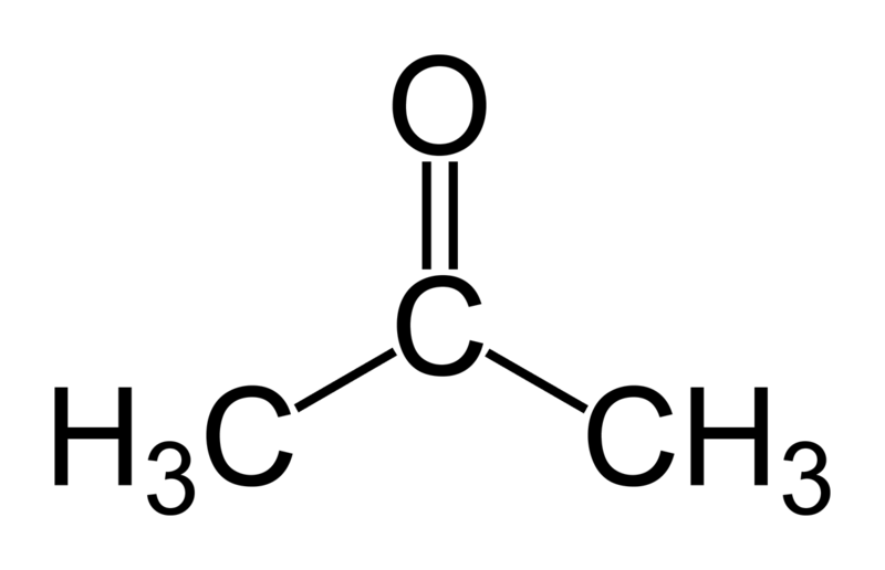
Figure 1 | Acetone (2-propanone) represented by a Na bead in the Martini force field.
Copy the 1_FreeSampling folder inside FreeEnergyTechniques on your desktop in which you will do the actual work. This prevents altering the original files by accident.
> cp -r FreeEnergyTechniques/1_FreeSampling .
Enter the folder you just copied and take a look at its content with a simple text editor.
> cd 1_FreeSampling/files_DoItYourself/1.1-intial
> gedit bead_template.itp
A general explanation of the format of .itp files can be found in the GROMACS manual. For now it is important to change the bead type of our single bead molecule (CG acetone) to the appropriate type. Do not forget to save after you have made your changes.
The em/eq/md.mdp files contain the settings for GROMACS. Things like the integrator type and time step, number of steps, pressure coupling scheme, electrostatic scheme, etc. For a full description of the .mdp settings you can take a look at the GROMACS manual.
The hexadecane_w.gro file contains the amount of beads, the coordinates of all the beads in your system and the dimensions (nm) of you periodicity. The dimensions can be found at the bottom of the file. The tail command can be used to only print the last few lines of a file.
> tail hexadecane_w.gro
We could try to count - by hand - all the water, hexadecane and acetone molecules but much easier would be to take a look at the topol.top file.
> gedit topol.top
The first lines of the .top file start with a # and here the locations of the forcefield parameters are specified. Then the system name is given an last the system composition is described. It is important to remember that the order of molecules in the .gro and .top should be exactly the same.
Before you close this file you should change the third line so it points towards your bead_template.itp. Do not forget to save your changes after you are done.
Inside the “top/” folder you will find the general .itp files of the Martini forcefield and the description for several solvents, including hexadecane.
To finalize our initial inspection of the system we will open it with vmd.
> vmd hexadecane_w.gro
By opening graphics/representations… from the main menu in vmd we can make some custom selections to improve our visualization. Some useful selections for now are:
resname W
resname HD
resname B
You can have multiple selections at the same time by clicking the Create Rep button in the top left of the same menu. Each selection has its own Drawing Method which can be selected from the drop-down menu in the bottom left of the same menu. A simple but effective Drawing Method is VDW, which shows each point as a sphere. Take your time to play a bit around with the visualization if you would like to. You can save your visualization by clicking file/Save Visualization State... from the main menu in vmd. You can close vmd by typing quit in the terminal.
> quit
By now we should know exactly what our system is and how to run it. We only have to do it! First, we need to energy minimize our system. To keep everything tidy we will start with making a separate folder for the minimization, equilibration, production and analysis run. Then we enter the just created em folder.
> mkdir em eq md analysis
> cd em
Now, we generate the em.tpr using gmx grompp and run it using gmx mdrun. The gmx points to the gmx toolbox containing many subroutines such as mdrun, which is the core md engine used by gromacs to perform the simulation. By only typing gmx, you can see all the other tools available. Many of them are for the analysis of md data. In most cases you can add the -h flag in any gmx command to get an overview of the available options for the requested subroutine (in the cases below this would be grompp and mdrun subsequently).
> gmx grompp -f ../em.mdp -c ../hexadecane_w.gro -p ../topol.top -o em.tpr
> gmx mdrun -deffnm em -v -rdd 2.0
After the simulation has finished successfully, we can enter the eq folder and perform some equilibration steps.
> cd ../eq
> gmx grompp -f ../eq.mdp -c ../em/em.gro -p ../topol.top -o eq.tpr
> gmx mdrun -deffnm eq -v -rdd 2.0
And finally we do the same for the production run:
> cd ../md
> gmx grompp -f ../md.mdp -c ../eq/eq.gro -p ../topol.top -o md.tpr
> gmx mdrun -deffnm md -v -rdd 2.0
The time it will take to finish the production run is stated in the last line during execution of gmx mdrun. This would be an excellent time to quickly grab a cup of coffee/thee/water and talk enthusiastically about molecular dynamics with your fellow students. A suitable topic could be 'Why don't we start with the production run right away?'. After this step you will start with the analysis to end up with a log(P) value which you can compare to the experimental value.
Now that the simulation has finished, it is time to perform the analysis. Move into the analysis folder which you created before and perform a density analysis for the simulation in the z dimension. To do so we will use gmx density. Like before you can gain extra information about this gmx tool by typing gmx density -h.
> cd ../analysis
> gmx density -f ../md/md.xtc -s ../md/md.tpr -center -symm -ng 3 -o density.xvg
You will be prompted to select the group for centering, selecting either the group representing W or HD should do. Then we would like to obtain the density for the W, HD and B seperately. Therefore select each one once (by typing the according number) followed by pressing return. After you have specified three groups the analysis will be performed. This should be finished within a matter of seconds. After the analysis has finished you can open the density.xvg file with xmgrace – a graphing program.
> xmgrace -nxy density.xvg
Though all the information is there, it is easier to look at after normalization. To do so you need to click at Data/Transformations/Evaluate Expression... in the main menu. In the popped up menu select all three sets on the left and all three sets on the right by dragging with your mouse. Now all sets on the left and right should have a black background. Next type y = y/max(y) in the Formula field and click Accept at the bottom center in the menu. All lines are now between 0 and 1, however our y-scale is still way too bloated. To quickly fix this you need to click the AS (auto scale) button in the general menu on the left (the second button on the right). Now find the y-value for B line in both the bulk W and HD (the x and y value of the center of you mouse are depicted underneath the main menu bar in the top left). You can calculate the log(Phexadecane-water) for acetone by dividing the HD-bulk population by the W-bulk population and then taking the logarithm of that fraction. Compare your value to the value published in the original paper [1,2]. By plugging in your acquired ratio for P in equation 1, you can obtain the free energy difference between the two states.
Assignments:
1) Think of some downsides for this technique.
2) For what kind of systems would you expect this technique to function well?
3) Continue with part 2, or help someone next to you and then continue with part 2.
Umbrella sampling
Frequently, unbiased MD simulations cannot be the appropriate technique to study systems involving rare events. Even in simple problems, as log(P) calculations, the sampling can be difficult. For example, solutes too hydrophobic could take a long time to visit the water phase. Increasing the solute concentration as a way to increase the frequency to happen these rare events has a limit: at some point you could induce solute aggregation or even changes in the solvent properties of the phases. If this is the case, special biased MD techniques can be used to improve the sampling. Here, we introduce the usage of one of the most traditional free energy methods, called Umbrella Sampling (US). In the US approach, the potential function – i.e. the interactions of your system – is modified in a way to equally sample favorable and unfavorable states along a reaction coordinate (RC). The RC is defined as the path between two well-defined states. We will apply the US approach to the same problem described in the previous part of the tutorial: hexadecane-water log(P) calculations of acetone (represented with a Na bead in the MARTINI coarse-grained force field). The main practical steps to obtain log(P) via US simulations are:
- Generate a series of initial configurations along the RC. In a water-hexadecane biphasic system, the most obvious RC is the position of your solute in the simulation box, from the bulk of one solvent to the bulk of the other one.
- Run US simulations on each configuration, restraining the solute in the center of the window via bias potentials. Often, harmonic potentials are used due to their simplicity.
- Use the weighted histogram analysis method (WHAM) to extract the potential of mean force (PMF) and calculate ΔGHD-W and log(PHD-W).
More details of the theory behind the US technique can be found in reference [3]. Hereafter, we describe step by step how to perform the US simulation. Now, let us start the hands-on section.
Generating the windows along the RC
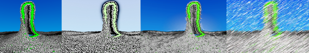
To perform US simulations, we must generate a series of configurations along the RC. These configurations will serve as the starting points for the US windows, which can be performed as parallel independent simulations. Figure 2 illustrates the principles: The top image illustrates the RC of the Na bead in the water-hexadecane biphasic mixture. We can start from water to hexadecane or vice versa, using the z-axis of the box as RC (x-axis in the image). The middle image corresponds to the independent simulations conducted within each sampling window along the RC, with the Na bead being restrained in that window by an umbrella biasing potential. The bottom images shows the ideal result as a histogram of configurations, with neighboring windows overlapping such that a continuous free energy function can later be derived from these simulations.
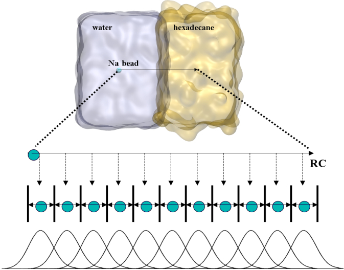
Figure 2 | Schematic view of protocol used in umbrella sampling.
To generate the initial configurations for each window, we need to perform a sequence of pulling, energy minimization and equilibration simulations. This protocol has been established based on trial-and-error to obtain a reasonable distribution of configurations. In other systems, it may be necessary to save configurations more often or even to apply a different minimization/equilibration procedure. The idea is to capture enough equilibrated configurations along the RC to obtain a regular spacing of the US windows (in terms of the Na distance position in z-axis from hexadecane to water).
Enter in the initial configuration folder and look at the files inside.
> cd FreeEnergyTechniques/2_UmbrellaSampling/files_DoItYourself/2.1.initial_configurations/
> ls
You will find a bash script (that will be commented on later), a .gro file and also some templates for the .mdp files. Theses files will be used to generate the initial conditions for each window of your RC. The start.gro file contains a CG model of hexadecane-water simulation box and 1 Na bead. Take a look in the system using vmd.
> vmd start.gro
The .mdp files are basically sequential steps of pulling, minimization and equilibration simulations. They were designed to smoothly put the Na bead in a specific position of your box (the windows along your RC). The position of Na is defined in the pulling parameters of the .mdp files. You can take a look at them (all parameters staring with pull) in one of the .mdp files using gedit.
> gedit em.mdp
You can find what these parameters control in the GROMACS manual. However, save this task for later, when you have started the production simulations. Now, create the folder for the first window and copy the .mdp files to this folder:
> mkdir 0.0/
> cp *.mdp 0.0/ (The * is a wildcard in bash, which is substituted for any amount of any character, therefore this copies all the .mdp files in one go. Pretty neat right?!)
Enter the 0.0 folder and modify in each .mdp file the pull-coord1-init parameter:
> cd 0.0/
> gedit <file>.mdp
Replace POS1 by 0.0 in each one of the .mdp files. Then generate the .tpr files and run the pulling, energy minimization and equilibration steps:
> gmx grompp -f pull.mdp -c ../start.gro -p ../../2.0.parameters/topol.top -o pull.tpr
> gmx mdrun -nt 1 -deffnm pull -v &> pullrun.log
> gmx grompp -f em.mdp -c pull.gro -p ../../2.0.parameters/topol.top -o em.tpr
> gmx mdrun -nt 1 -deffnm em -v &> emrun.log
> gmx grompp -f em2.mdp -c em.gro -p ../../2.0.parameters/topol.top -o em2.tpr
> gmx mdrun -nt 1 -deffnm em2 -v &> em2run.log
> gmx grompp -f eq.mdp -c em2.gro -p ../../2.0.parameters/topol.top -o eq.tpr
> gmx mdrun -nt 1 -deffnm eq -v -px eq_x -pf eq_f &> eqrun.log
Repeat the procedure for each other window, from 0.1 to 3.9, with spacing of 0.1 nanometer. As you already know how the whole procedure works, you can use a bash script to automatically generate all other 39 windows. First come back to the parent folder and then run the script.
> cd ../
> ./initial_configurations.sh
Running the production simulations for each window
Enter in the production folder and look at the files inside:
> cd ../2.2.production/
> ls
Now, run the US simulations. As in the previous step, you should now generate folders for each window and perform longer production simulations. We separate this task with two scripts, to run two sets of simulations in parallel.
> nohup ./umbrella1.sh & (The & sign is to cast the process to the background. nohup makes sure that even when you close the current terminal, the process remains active.)
> nohup ./umbrella2.sh &
This step should take a maximum of 30 minutes. In the mean time, take a look at the GROMACS manual to find the meaning of all pulling parameters used in the .mdp files. If you have questions, ask your neighbours, or talk with one of the supervisors (or both). You can also take a look at the recommended reference about US.
In case some problems occur and you do not manage to finish the US simulations within approx. 1 hour, please use the files in the directory files_worked to perform the analysis. However, if your simulation is taking longer than the stated amount of time, it is always good to notify a supervisor of your problem.
Data analysis
The most common analysis conducted for US simulations is the extraction of the PMF, which will yield the hexadecane-water partition ΔG for the Na partition. ΔG is simply the difference between the water and hexadecane values of the PMF curve (similar as performed in the previous tutorial). A common method for extracting PMF is the WHAM, included in Gromacs as the wham utility. Its input consists of two files, one lists the names of the production .tpr files of each window, and the other that lists the names of either the pullf.xvg or pullx.xvg files from each window. First, enter the data analysis folder and generate the files containing the list of production .tpr and pullx.xvg files:
> cd ../2.3.analysis/
> ls -d ../2.2.production/*/md.tpr > tpr-files.dat
> ls -d ../2.2.production/*/md_x.xvg > pullx-files.dat
Then, run the gromacs tool wham:
> gmx wham -ix pullx-files.dat -it tpr-files.dat -bsres -bins 200 -temp 300 -unit kJ -b 100 -nBootstrap 100 -zprof0 3.5 -min 0 -max 3.9
The WHAM utility will open each of the umbrella.tpr and pullx.xvg files sequentially and run the WHAM analysis on them. Take a look in the meaning of the other input parameters used to run gmx wham using its help option (gmx wham -h). For example, the -unit kJ option indicates that the output will be in [kJ/mol], but you can also get results in [kcal/mol] or [kBT]. After running gmx wham, you should end up with a profile.xvg file that looks similar to Figure 3A, except it does not show the error bars. You can open the result using xmgrace.
> xmgrace profile.xvg
If you want to see the error bars (and this is recommended!) inspect the file bsResult.xvg. All individual profiles from the bootstrapping are in the file bsProfs.xvg. One of the other outputs of the wham command will be a file called histo.xvg, which contains the histograms of the configurations within the US windows. These histograms will determine whether or not there is sufficient overlap between adjacent windows. For the types of simulations conducted as part of this tutorial, you may obtain something like Figure 3B. The histograms have to show reasonable overlap between the sampled windows.
> xmgrace -nxy histo.xvg
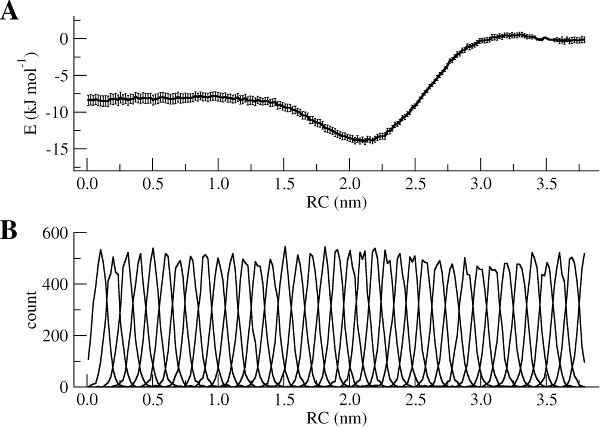
Figure 3 | (A) PMF of the Na bead from bulk water (RC = 0 nm) to hexadecane (RC = 3.8 nm). (B) Histograms of the positions of a Na bead in each window.
Assignments
1) Calculate the partition coefficient of the Na bead and compare it with the values you calculated with the free sampling approach and with the experimental value in the literature.
2) What are the advantages and disadvantages of umbrella sampling in relation to the free sampling method?
3) How can you make sure that your simulations reached convergence?
4) Continue with part 3, or help someone next to you before continuing with part 3.
Thermodynamic integration
The calculation can be performed in several ways, but we will do it here by integrating the average derivative of the Hamiltonian (read: interaction potential) with respect to the coupling parameter in a piecewise fashion, i.e. calculate the average derivative with respect to the coupling parameter at a set of values of the coupling parameter and integrate it. Fortunately, Gromacs will take care of all these complicated calculations. An important issue to be addressed is the convergence of the final integrated number. The convergence depends on the error in the averages at the different λ points and on the smoothness of the curve, i.e. the number of individual λ points used in the integration. This will require a lot of simulations and therefore a number of results will be provided to you in case you ran out of time. However, first one needs to set up the systems at individual λ points. We will set up an individual λ point for solvation of a Na bead (NOTE: not a sodium ion, but an N-type bead with hydrogen-bond acceptor properties) in water, and then use a bash script to set up and run simulations pertaining to all λ points in parallel. You will also prepare a set-up for calculating solvation free energy of a Na bead in hexadecane following the same steps as the set up in water.
Setting up the solvated system of a Na bead in water
The initial files for this exercise are provided in the subdirectory 3_ThermodynamicIntegration/files_DoItYourself/SETUPINWATER.
In order to perform a (classical mechanical molecular dynamics) simulation, the system and the simulation conditions need to be specified. Gromacs implements these specifications in three files: the topology file specifies the molecules in the system, the coordinate file specifies the starting coordinates (and velocities) of the atoms, and the run parameter file specifies the simulation control variables (number of steps, time step, output frequency, etc.). We will first quickly get the simulation running, then will focus on specific issues relating to free energy calculations.
Topology
The topology file (standard extension .top, standard name topol.top) specifies the number and types of particles (used interchangeably with atoms in the remainder of this document) in the system. Note that the topology file may specify that there are multiple copies of the same molecule in the system; thus, the amount of information to be specified may be greatly reduced because details for each type of molecule need to be specified only once.
For this exercise, the perturbation topology of Na bead is already given in the file topol.top.
Open the file topol.top from the directory SETUPINWATER in an editor. You will notice that the topology file seems to contain very little information. The structure of the file is briefly described below.
A. First the force field is specified. The force field used in this exercise is the martini force field. The master file is called martini.itp and it is read by the preprocessor because of the #include statement.
B. and C. The second file included in the topology file is called martini_na.itp, which contains the definition of the Na molecule, including the description required for the alchemical transformation that enables calculation of the solvation free energy. The third file included in the topology file is called martini_solvents.itp, which contains the definition of the water and hexadecane molecules. The order of these two files is not important. If your system contains more types of molecules, for example ions, you can add include an .itp file for each of them.
D. Each system needs a specification describing the system. This information is printed in some output files and may be useful for you to identify the system you are working on. In general, it is always wise to have a SEPARATE directory for EACH simulation system. You may easily get confused!
E. All that remains to be done in the topology file topol.top is to specify the number of molecules in the system. You need one line for each type of molecule. The order in which you specify the molecules is important. The Na bead is elsewhere specified with a molecule name Na, and the name for the water and hexadecane molecule is W and HD, respectively. The program interprets the starting coordinates (see next section) as belonging to the molecules in the order you specify here. It does NOT check the names of the molecules! We do not know the number of water molecules yet, because we need to first solvate the Na molecule. We will make sure to have 1280.
Starting coordinates and velocities
GROMACS takes a number of formats for input coordinates (and velocities). For this exercise, the simple “in-house” format is used. The standard file extension is .gro. The file Na.gro contains starting coordinates for a single Na bead. Note that the first line is a descriptive text, the second line contains the number of atoms in the system, and the last line contains the dimensions of the simulation unit cell.
The Na molecule first needs to be solvated. The GROMACS tools insert-molecules and solvate can add coordinates of molecules to existing coordinates, taking care that individual atoms are not too close together. The tool insert-molecules takes a single molecule to be added, puts its center-of-mass randomly somewhere in the box defined in the existing molecule (dimensions of the box are specified on the last line of the .gro file) and randomly rotates the new molecule. It then checks for clashes with previously present molecules and only inserts the new molecule if no such clashes are present. One may repeatedly use this procedure to insert a number of solvent molecules. However, one may also add solvent molecules when a box of solvent is available, by using the tool solvate. For solvation in water, a box containing 2704 W beads is provided (solvent.gro). If this equilibrated box is provided with the option –cs, solvate does not rotate this box, but fills the space with periodic replicas and then checks the individual molecules for clashes so that it does not reject all molecules if only one of them clashes.
Make sure you have the terminal running and are in the correct directory SETUPINWATER. Solvate the Na bead:
> gmx solvate –cp Na.gro –cs solvent.gro -o solvated.gro -box 5.5 5.5 5.5 -maxsol 1280
There should be no more than 1280 W beads added to the original box. If not, please try to solvate again in such a way that you end up with 1280 W beads (you can try a different seed for the random number). It is important that you use the same number of water molecules in these exercises (or the results obtained for TI calculations cannot be compared to previous sections)!
The final ingredient for a simulation are the run parameters, with standard extension .mdp.
In this exercise, we will need to perform two types of runs:
A. energy minimization of the solvated system
B. free energy calculation at single λ point
The engine to run the simulation is mdrun. The program mdrun requires one (binary) input file containing all information required to run the simulation. The standard name for the run input file is topol.tpr, and it is generated using the GROMACS program gmx grompp, which takes the .top, .gro, and .mdp files discussed in the previous section.
Run the preprocessor
> gmx grompp –p topol.top –c solvated.gro –f min.mdp -o min -maxwarn 2
Check that you have generated a file called min.tpr. If not, the step may have failed because of ERRORS or because of WARNINGS. The warnings can usually be ignored (maybe check with your assistant if you’re not sure), ERRORS need to be fixed. Try to figure out what was wrong and fix it. The file min.tpr. is readable by the GROMACS engine and contains all necessary information. You can run the engine using this min.tpr file by typing the command
> gmx mdrun –v -deffnm min
If all is well, you should now have produced a good starting structure for calculation of derivative of the energy at the single λ point. By default it will be written in the file min.gro. Copy this file to a new directory (production directory, see next section) and rename it start.gro to set up the simulation generating the required data for the single λ point. To this directory, also copy all .itp files, the .top file, and the file run.mdp.
Setting up a perturbation simulation at a particular value of the coupling parameter
Run parameters for a single λ point
Create a directory for production run and go there:
> mkdir production
> cd production
Remember to copy the files you need to this directory! The file run.mdp contains the settings for a single λ point. Open the file run.mdp in an editor. Note the following settings :
Control parameters for free energy calculation. This is the core of the present exercise.
First of all, we specify free-energy = yes to ensure calculation of dH/dλ. The value of λ is given by init-lambda and should be different for each lambda point. In the exercise, check that the value of λ is 0.
When switching on/off non-bonded interactions, atoms can be quite close to each other, much closer than in fully interacting systems. To avoid large forces or dH/dλ values, soft core potentials are used instead of the LJ potential. Soft core potentials have the property that their value is finite at distance 0. For the MARTINI force field, values of sc-alpha = 0.5 usually perform well.
The parameter sc-power controls the rate at which the coupling varies with λ. With sc-power = 1 the change in interaction is linear in λ, sc-power = 2 specifies quadratic change.
Running a single λ point
All is now in place to run a simulation. Therefore, now execute the following commands
> gmx grompp –p topol.top –c start.gro –f run.mdp -o run
Check that you have generated a file called run.tpr. If not, the step may have failed because of ERRORS or because of WARNINGS. The warnings can usually be ignored (maybe check with your assistant if you’re not sure), ERRORS need to be fixed. Try to figure out what was wrong and fix it. The file run.tpr. is readable by the GROMACS engine and contains all necessary information. Run the engine using this run.tpr file by typing
> gmx mdrun -deffnm run >& run.job &
If all is well, you should now be producing data to give you an estimate of the dH/dλ at the λ point. The next task is to compute the change in free energy by integrating the entire dH/dλ curve as a function of λ. Check that sensible data are produced by looking at the file run.xvg.
> tail run.xvg
If sensible data (i.e. numbers, not inf or nan) are being produced, proceed to have a close look at the details of this simulation. NOTE that it may take a while before the first data appear in run.xvg.
Running all λ points
In order to quickly produce all of the input files needed for running simulations for each value of λ points, we have made a bash script available. Make a new directory called production_all
> mkdir production_all
> cd production_all
and copy min.mdp, topol.top,.itp , run2.mdp,solvent.gro, TI.sh and Na.gro to this directory. Have a look at the script TI.sh . You may need to change some commands, in particular the loading of GROMACS, depending on your computer. If you are satisfied that the commands are correct, proceed to executing the script. To issue the bash script:
> ./TI.sh
The script will create directories with relevant values of init_lambda_state inserted to the run2.mdp file and will proceed to execute TI calculation for each state. This means that for each value of λ, minimization and production steps will be performed in separate directories. To analyze the data, GROMACS bar module will be used to conduct Bennett acceptance ratio (BAR) method and compute free energy of solvation. The bar module will collect all the .xvg files that were generated ( for each value of λ ) and produce three output files; bar.xvg, barint.xvg and histogram.xvg. The value of solvation free energy will be printed in a .dat file named final.dat.
Assignments:
1) How would you make sure about the convergence of the simulations? Maybe have a look at .xvg files produced at the final stage of the simulations.
2) Can you make a statement about what is a reasonable simulation time for each λ point?
3) What might be good strategies to get a small error in the solvation free energy? Think about the balance between increasing the number of λ points and the length of simulation at a single λ point. If you were to increase simulation of a single λ point, which λ would you pick?
Setting up the solvated system of a Na bead in hexadecane
In Exercise 2, the solvation free energy of solvation of a Na bead in hexadecane is calculated using TI. The directory S3_ThermodynamicIntegration/files_DoItYourself/ETUPINHD contains the required files. Enter that directory.
Follow the steps described for the set up in water. For HD solvent, you should change the number of solvent molecules using the following command:
> gmx solvate -cp Na.gro -cs solvent.gro -o solvated.gro -box 5.5 5.5 5.5 -maxsol 320
and then continue with the rest of the set up as stated above for solvation of Na bead in water.
For each state, run a minimization and production simulation using TI.sh .
Assignments:
1) What is the solvation free energy change of the Na bead in water and hexadecane?
2) Calculate the partition coefficient of Na bead and compare it with the values you calculated with other methods and with the experimental value in the literature? What is the source of difference?
3) Which method is the most efficient one to calculate partition coefficient in the current system? What if you had a more complicated system?
4) Can you find other application for TI method other than the ones specified in the tutorial?
References
[1] Marrink, S. J., De Vries, A. H., and Mark, A. E. (2004) Coarse grained model for semiquantitative lipid simulations. J. Phys. Chem. B 108, 750–760.
[2] Marrink, S. J., Risselada, H. J., Yefimov, S., Tieleman, D. P., and De Vries, A. H. (2007) The MARTINI force field: coarse grained model for biomolecular simulations. J. Phys. Chem. B 111, 7812–7824.
[3] Kästner, J. (2011) Umbrella sampling, WIREs: Comp. Mol. Sci. 1, 932–942.