


Martini tutorials: proteins
- Details
- Last Updated: Tuesday, 18 August 2015 08:26
Martini tutorials: proteins
(if you just landed here, we recommend you follow the tutorial about lipid bilayers first)
Summary
Soluble protein: the Martini description
Soluble protein: the elastic network approach
To go further: membrane protein
Tools and scripts used in this tutorial
Soluble protein
Keeping in line with the overall Martini philosophy, the coarse-grained protein model groups 4 heavy atoms together in one coarse-grain bead. Each residue has one backbone bead and zero to four side-chain beads depending on the residue type. The secondary structure of the protein influences both the selected bead types and bond/angle/dihedral parameters of each residue[1]. It is noteworthy that, even though the protein is free to change its tertiary arrangement, local secondary structure is predefi ned and thus imposed throughout a simulation. Conformational changes that involve changes in the secondary structure are therefore beyond the scope of Martini coarse-grained proteins.
Setting up a coarse-grained protein simulation consists basically of three steps:
1. converting an atomistic protein structure into a coarse-grained model;
2. generating a suitable Martini topology;
3. solvate the protein in the wanted environment.
Two first steps are done using the publicly available martinize.py script, of which the latest version can be downloaded here. The last step can be done with the tools available in the gromacs package and/or with ad hoc scripts. In this part of the tutorial, some basic knowledge of gromacs commands is assumed and not all commands will be given explicitly. Please refer to the previous tutorials (basic tutorial on Martini lipids available here) and/or the gromacs manual.
The aim of the first module of this tutorial is to define the regular work flow and protocols to set up a coarse-grained simulation of ubiquitin in a water box using a standard Martini description. The second module is presenting the variation of the secondary structure which can occur for certain proteins, in our case the HIV-1 protease, and a slightly different approach to avoid this issue. The last module is to set up a coarse-grained simulation of a KALP peptide in its membrane environment.
Soluble protein: the Martini description
Download all the files of this module
The downloaded file is called ubiquitin.tgz and contains the worked version of this module. You can use this worked version to check your own work. The file expands to the directory soluble-protein; the files for this module are in the directory ubiquitin/martini. Create your own directory to work the tutorial yourself. Instructions are given for files you need to download, etc. You do not need any files to start with. Now go to your own directory.
After getting the atomistic structure of ubiquitin (1UBQ), you'll need to convert it into a coarse-grained structure and to prepare a Martini topology for it. Once this is done the coarse-grained structure can be minimized, solvated and simulated. The steps you need to take are roughly the following:
1. Download 1UBQ.pdb from the Protein Data Bank.
$ wget http://www.rcsb.org/pdb/files/1UBQ.pdb.gz
$ gunzip 1UBQ.pdb.gz
2. The pdb-structure can be used directly as input for the martinize.py script (download available here), to generate both a structure and a topology file. Have a look at the help function (i.e. run martinize.py -h) for the available options. Hint, valid for any system simulated with Martini: during equilibration it might be useful to have (backbone) position restraints to relax the side chains and their interaction with the solvent; we are anticipating doing this by asking martinize.py to generate the list of atoms involved. The final command might look a bit like this:
$ martinize.py -f 1UBQ.pdb -o system-vaccum.top -x 1UBQ-CG.pdb -dssp /path/to/dssp -p backbone -ff martini22
We are asking for version 2.2 of the force field. When using the -dssp option you'll need the dssp binary, which determines the secondary structure classification of the protein backbone from the structure. It can be downloaded from the CMBI website. As an alternative, you may prepare a file with the required secondary structure yourself and feed it to the script:
$ martinize.py -f 1UBQ.pdb -o system-vaccum.top -x 1UBQ-CG.pdb -ss <YOUR FILE> -p backbone -ff martini22
Note that the martinize.py script might not work with older versions of python! Also python 3.x migth not work. We know it does work with versions: 2.6.x, 2.7.x and does not work with 2.4.x. If you have tested it with any version in between, we would like to hear from you.
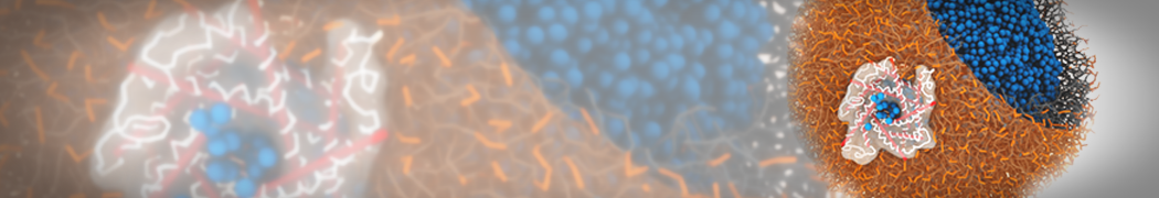
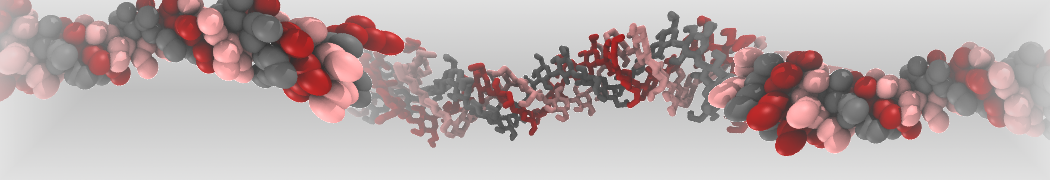
3. If everything went well, the script generated three files: a coarse-grained structure (.gro/.pdb; cf. Fig. 1), a master topology file (.top), and a protein topology file (.itp). In order to run a simulation you need two more: the Martini topology file (martini_v2.x.itp, if you specified version 2.2, you'll want the corresponding file) and a run parameter file (.mdp). You can get examples from the Martini website or from the protein tutorial package. Don't forget to adapt the settings where needed!
A B
B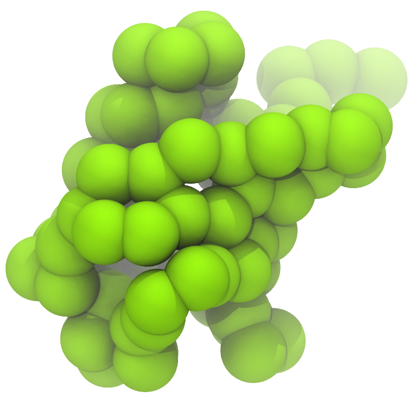 C
C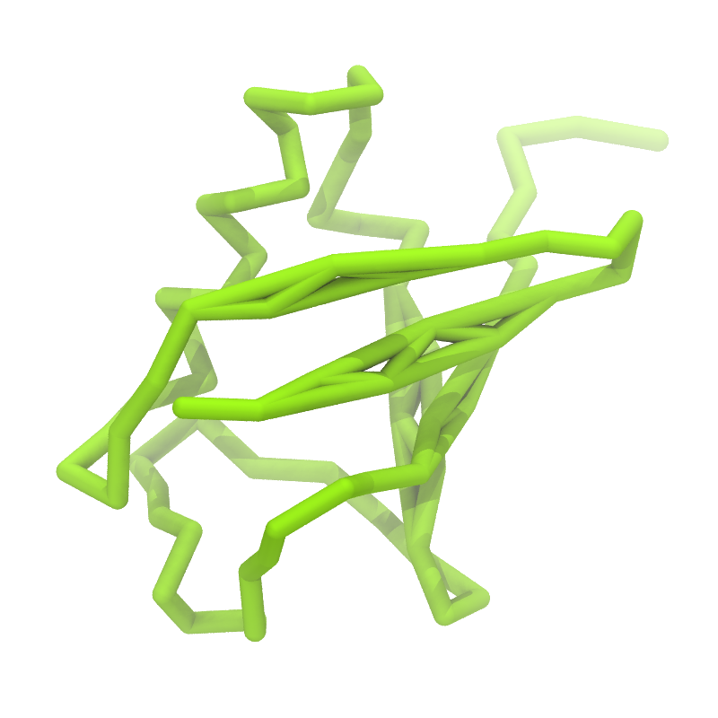
Figure 1 | Different representations of ubiquitin. A) cartoon representation of the atomistic structure. B) Coarse-grained beads forming the backbone and C) licorice representation of the backbone of the martinized protein.
4. Do a short (ca. 10 steps is enough!) minimization in vacuum. Before you can generate the input files with grompp, you will need to check that the topology file (.top) includes the correct martini parameter file (.itp). If this is not the case, change the include statement. Also, you may have to generate a box, specifing the dimensions of the system, for example using editconf. You want to make sure, the box dimensions are large enough to avoid close contacts between periodic images of the protein, but also to be considerably larger than twice the cut-off distance used in simulations. Try allowing for a minimum distance of 1 nm from the protein to any box edge. Then, copy the example parameter file, and change the relevant settings to do a minimization run. Now you are ready to do the preprocessing and minimization run:
$ editconf -f 1UBQ-CG.pdb -d 1.0 -o 1UBQ-CG.gro
$ grompp -f minimization-vaccum.mdp -p system-vaccum.top -c 1UBQ-CG.gro -o minimization-vaccum.tpr
$ mdrun -deffnm minimization-vaccum -v
5. Solvate the system with genbox (an equilibrated water box can be downloaded here; it is called water.gro, in the command below, it is saved as water-box-CG_303K-1bar.gro). Make sure the box size is large enough (i.e. there is enough water around the molecule to avoid periodic boundaries artifacts) and remember to use a larger van der Waals distance when solvating to avoid clashes, e.g.:
$ genbox -cp minimization-vaccum.gro -cs water-box-CG_303K-1bar.gro -vdwd 0.21 -o system-solvated.gro
6. Do a short energy minimization and position restrained simulation of the solvated system. Since the martinize.py script already generated position restraints (thanks to the -p flag), all you have to do is specify define = -DPOSRES in your parameter file (.mdp) and add the appropriate number of water beads (the molecule name is W) to your system topology (.top); the number can be seen in the output of the genbox command.
$ grompp -f minimization.mdp -c system-solvated.gro -p system.top -o minimization.tpr
$ mdrun -deffnm minimization -v
$ grompp -f equilibration.mdp -c minimization.gro -p system.top -o equilibration.tpr
$ mdrun -deffnm equilibration -v
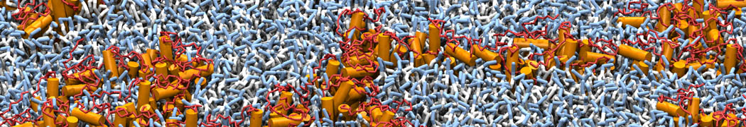
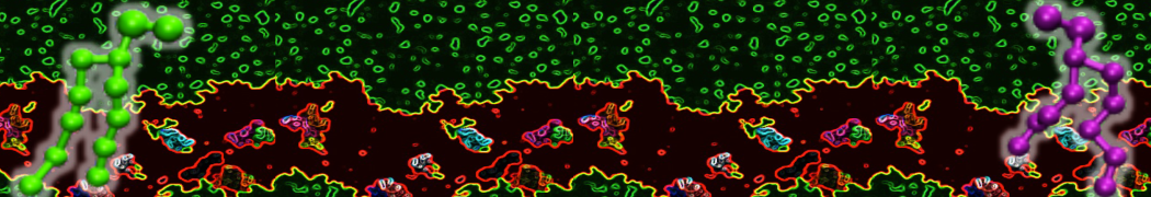
7. Start production run (without position restraints!); if your simulation crashes, some more equilibration steps might be needed. A sample trajectory is shown in Figure 2.
$ grompp -f dynamic.mdp -c equilibration.gro -p system.top -o dynamic.tpr
$ mdrun -deffnm dynamic -v
Figure 2 | 20 ns simulation of coarse-grained ubiquitin (green beads) and solvent (coarse-grained water; blue beads).
8. PROFIT! What sort of analysis can be done on this molecule? Start by having a look at the protein with vmd.
Soluble protein: the elastic network approach
Download all the files of this module
The aim of this second module is to see how application of elastic networks can be combined with the Martini model to conserve secondary, tertiary and quartenary structures more faithfully without sacrificing realistic dynamics of a protein. We offer two alternative routes. Please be advised that this is an active field of research and that there is as of yet no "gold standard". The first option is to generate a simple elastic network on the basis of a standard Martini topology. The second options is to use an ElNeDyn network. This second option constitutes quite some change to the Martini force field and thus is a different force field in itself. The advantage is that the behavior of the method has been well described[2]. Both approaches can be set up using the martinize.py script and will be shortly described below.
We recommend to simulate a pure Martini coarse-grained protein (without elastic network) in a first step, and then see what changes are observed when using an elastic network on the same protein. Note that you'll need to simulate the protein for tens to hundreds of nanoseconds to see major changes in the structure; sample simulations are provided in the archive.
Martini
1. Repeat steps 1 to 7 from the previous exercise with the HIV-1 protease (1A8G.pdb).
2. Visualize the simulation, look especially at the binding pocket of the protein: does it stay closed, open up? What happens to the overall protein structure?
Martini + elastic network
The first option to help preserve higher-order structure of proteins is to add to the standard Martini topology extra harmonic bonds between non-bonded beads based on a distance cut-off. Note that in standard Martini, long harmonic bonds are already used to impose the secondary structure of extended elements (sheets) of the protein. The martinize.py script will generate harmonic bonds between backbone beads if the options -elastic is set. It is possible to tune the elastic bonds (e.g.: make the force constant distance dependent, change upper and lower distance cut-off, etc.) in order to make the protein behave properly. The only way to find the proper parameters is to try different options and compare the behavior of your protein to an atomistic simulation or experimental data (NMR, etc.). Here we will use basic parameters in order to show
the principle.
1. Use the martinize.py script to generate the coarse-grained structure and topology as above. For the elastic network, use the extra following flags:
$ martinize.py [...] -elastic -ef 500 -el 0.5 -eu 0.9 -ea 0 -ep 0
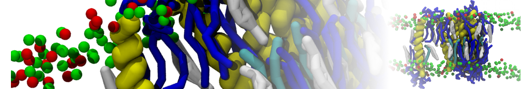
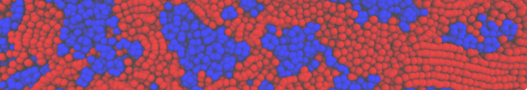
This turns on the elastic network (-elastic), sets the elastic bond force constant to 500 kJ.mol-1.nm-2 (-ef 500), the lower and upper elastic bond cut-off to 0.5 and 0.9 nm, respectively (-el 0.5 and -eu 0.9), and makes the bond strengths independent of the bond length (elastic bond decay factor and decay power, -ea 0 and -ep 0, respectively; these are default). The elastic network is defined in the .itp file by an #ifdef statement, and is switched on by default (#define NO_RUBBER_BANDS in the .top or .itp file switches it off). Note that martinize.py does not generate elastic bonds between i → i+1 and i → i+2 backbone bonds, as those are already connected by bonds and angles (cf. Fig. 3).
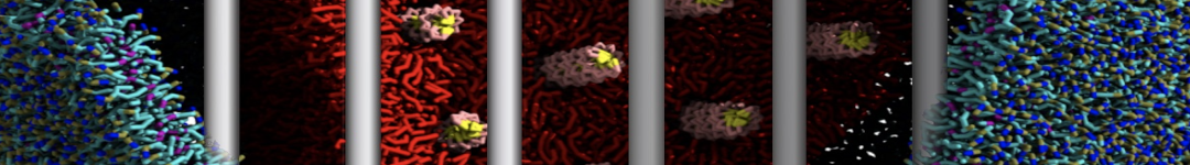
Figure 3 | Elastic network (gray) applied on the both monomer of the HIV-1 protease (yellow and orange, respectively)
2. Proceed as before (steps 4 to 7) and start a production run. Keep in mind we are adding a supplementary level of constraints on the protein; some supplementary relaxation step might be required (equilibration with position restraints and smaller time step for instance).
ElNeDyn
The second option to use elastic networks in combination with Martini puts more emphasis on remaining close to the overall structure as deposited in the PDB than standard Martini does. The main difference from the standard way (used in the previous exercise) is the use of a global elastic network between the backbone beads to conserve the conformation instead of relying on the angle/dihedral potentials and/or local elastic bonds to do the job. The position of the backbone beads is also slightly different: in standard Martini the center of mass of the peptide plane is used as the location of the backbone bead; but in the ElNeDyn implementation the positions of the Cα-atoms are used instead. The martinize.py script automatically sets these options and sets the correct parameters for the elastic network. As the elastic bond strength and the upper cut-off have to be tuned in an ElNeDyn network, these options can be set manually (-ef and -eu flags); note however these parameters have been extensively studied and were optimized to 500 kJ.mol-1.nm-2 and 0.9 nm[2].
1. Use the martinize.py script to generate the coarse-grained structure and topology as above. The following flag will switch martinize.py to the ElNeDyn default representation:
$ martinize.py [...] -ff elnedyn22
2. Proceed as before and start a production run.
Now you've got three simulations of the same protein with different type of elastic networks. If you do not want to wait, some pre-run trajectories can be found in the archive. One of them might fit your needs in terms of structural and dynamic behavior. If not, there are an almost infinite number of ways to further tweak the elastic network!
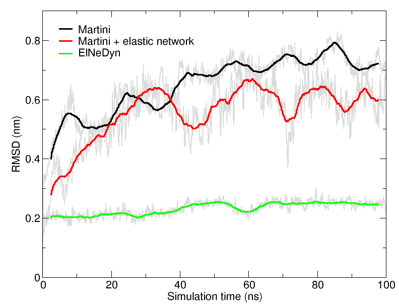
Figure 4 | RMSD of HIV-1 protease backbone with the three different approaches described previously (RMSD is usually considered "reasonnable" if below 0.3 nm).
An easy way to compare the slightly different behaviors of the proteins in the previous three cases is to follow deviation/fluctuation of the backbone during simulation (and compare it to an all-atom simulation if possible). RMSD (Fig. 4) and RMSF can be calculated using gromacs tools. vmd provides also a set of friendly tools to compute these quantities, but needs some tricks to be adapted to coarse-grained systems (standard keywords are not understood by vmd on coarse-grained structures).
To go further: membrane protein
Download all the files of this module (worked with old-style lipid collection topology file)
Download the minimum set of files for this module and set everything up yourself using the lipidome topologies
In the last module of this protein tutorial, we will increase the complexity of our system by embedding the protein in a lipid bilayer (the tutorial on old-style lipid bilayer can be followed here and the tutorial using the lipidome is here). We propose here to have a look at the tilt and the dimerization of KALP peptides embedded in DPPC membrane. The coarse-grained structure (kalp.gro) and topology (kalp.itp) of KALP are given in the archive; no need to repeat steps 1 to 4 martinizing the peptide from above. We will start here from step 5 since we are going to use a different way of solvating the proteins. Many different options to perform this step are available to us; a non-exhaustive list, ordered by decreasing complexity, is presented below:
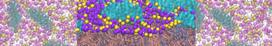
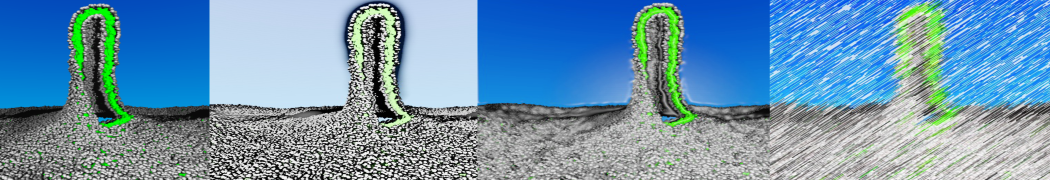
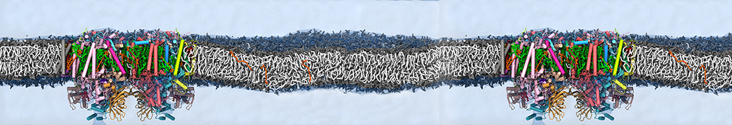
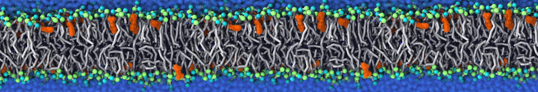
- A bilayer self-assembly dynamic, as presented in the first module of the lipid tutorial, will result in the self-insertion of the WALP inside the bilayer (Fig. 5).
A
B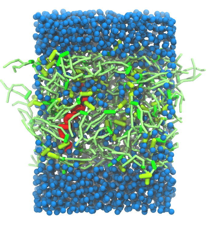 C
C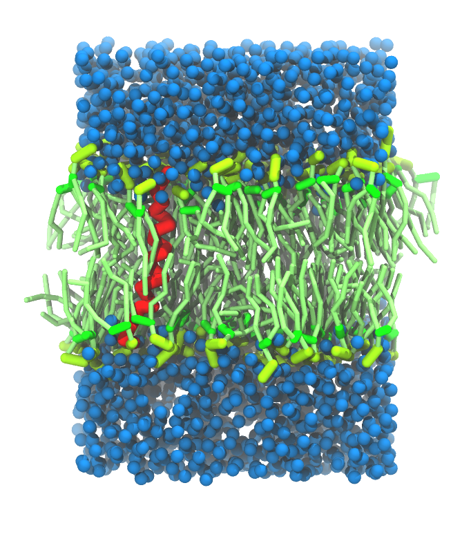
Figure 5 | A) Self-assembly (4 ns) of a DPPC (green) bilayer embedding a KALP peptide. B) Initial "soup" of lipid and solvent (water; blue) in which the KALP (red) is mixed. C) Final conformation of the simulation.
- If a stable DPPC membrane with the wanted box dimensions is already available, genbox will be able to insert the peptides in the bilayer (the peptides have to be pre-centered and positioned to ensure their presence inside the membrane).
- The use of the script insane.py, downloadable here.
The latter allows the insertion of a protein in a bilayer with any composition. Being the easiest and the most straightforward, we recommend this way of doing and that is what we are presenting here.
1. The syntax of the insane.py scripts is very similar to what was used so far; it can be invoked by running insane.py -h. Let's see a practical example:
$ insane.py -f kalp.gro -o system.gro -p system.top -pbc square -box 10,10,10 -l DPPC -center -sol W
The previous command line will set up a complete system, containing a squared DPPC bilayer of 10 nm, insert the KALP peptide centered in this bilayer and solvate the whole thing in standard coarse-grained water. More on the insane.py tool can be found in separate tutorials, notably setting up a complex bilayer. (with old-style lipids here).
2. Proceed as before and start a production run. To remind you, this involves (1) editing the system.top file to reflect the version of Martini you want to use (the KALP topology provided is version 2.1) and providing include statements for the topology files; (2) downloading or copying definitions of Martini version you want and the DPPC lipid topology file from the lipidome; (3) using the correct names of the molecules involved; (4) downloading or copying set-up .mdp files for minimization, equilibration, and production runs and if necessary, editing them (bilayer simulations are best done using semi-isotropic pressure coupling and you may want to separately couple different groups to the thermostat(s)); (5) running the minimization and equilibration runs.
3. Generate a new system in which membrane thickness is reduced (different the lipid type, DLPC for instance). Observe how the thickness is affecting the tilt of the transmembrane helix; compare it to the previous simulation.
4. Double these previous boxes in one dimension (genconf) and rerun the simulations. Observe the different dimerization conformations (parallel or anti-parallel tilts). Note that more than one simulation might be required to observe both cases!
5. Choose your favorite orientation and reverse-map the last conformation (tutorial on reverse-mapping available here). Simulate this system atomistically to refine and have a closer and detailed look at the interactions between KALPs.
Tools and scripts used in this tutorial
gromacs (http://www.gromacs.org/)
martinize.py (downloadable here)
insane.py (downloadable here)
[1] L. Monticelli, S.K. Kandasamy, X. Periole, R.G. Larson, D.P. Tieleman, S.J. Marrink. The MARTINI coarse grained forcefield: extension to proteins. J. Chem. Theory Comput., 4:819-834, 2008.
[2] X. Periole, M. Cavalli, S.J. Marrink, M.A. Ceruso. Combining an elastic network with a coarse-grained molecular force field: structure, dynamics, and intermolecular recognition. J. Chem. Theory Comput., 5:2531-2543, 2009.