


Martini tutorials: visualizing Martini systems using VMD
VMD is a molecular visualization program for displaying, animating, and analyzing large biomolecular systems using 3-D graphics and built-in scripting. (http://www.ks.uiuc.edu/Research/vmd/).
In this module, we explain some of the vmd commands that can be used to visualize the CG systems. Additionally, Tcl scripts are presented that assist with the visualization of CG systems; these scripts, as well as extended help, are available on the Martini website
An additional, very usefull tool for displaying CG (Martini) structures in VMD is Bendix. A good tutorial for Bendix can be found here:
http://sbcb.bioch.ox.ac.uk/Bendix/
Some basics
VMD adopted a representation-philosophy: for any set of atoms/molecules/protein chains we want to display or analyze, we need to select this set through a "representation" de fined by keywords related to this set (somewhat similar to make_ndx). VMD comes with implemented keywords for all-atom systems ("protein", "chain", "hydrogen", "solvent", etc.). More general keywords are implemented to be able to display non-classical-systems (CG systems are part of this second category); you can fi nd them in VMD manual:
http://www.ks.uiuc.edu/Research/vmd/current/ug/
Below are listed a few examples:
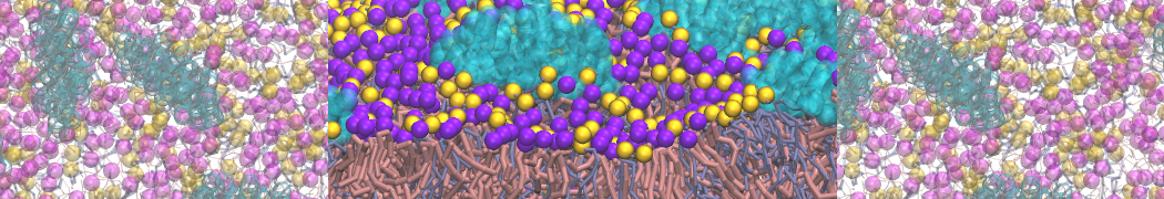
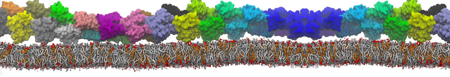
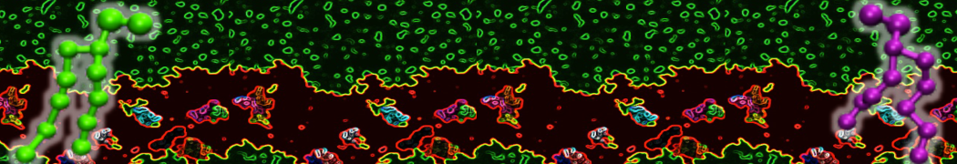
- To select only lipids: resname POPC, or only part of each lipids: resname POPC and name "C.*.A" "C.*.*.B" "D.*.A" "D.*.B" for lipid tails (C1A,C1B, etc.) and resname POPC and name NC3 PO4 "GL.*" for heads.
- To select only backbone beads of a protein: name BB (use "BB.*" or BAS for old versions of FG-to-CG scripts).
- To get rid of solvent (water/ion beads): not resname W WF ION or WP in case of polarizable water.
- To show only charged positively charged residues (in Martini): resname LYS ARG.
- To display the water shell around speci c residues: within 7.0 of (index 531 to 538).
- To display all lipids (excluding DPPC) whose heads are interacting with the same speci fic residues: same resid as ((within 7.0 of (index 531 to 538)) and name NC3 PO4 "GL.*") and not resname DPPC.
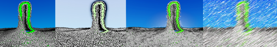
As you can see in the examples, all these keywords can be mixed with the logical links: and, or, not, etc. to produce any representation. Try it yourself! VMD is really demanding in term of memory; an easy trick to decrease the amount needed by VMD is to load structure/trajectories containing only beads needed by your analysis; this can easily be done by preprocessing the trajectory using trjconv. And as we are simulating bigger and bigger systems in which more and more beads are involved, the previous trick can be adapted to increase the displaying/seeking speed of trajectories by writing representations showing only beads needed for the visualization (head groups of a bilayer for instance). Keep in mind that you can save the visualizing state of your system whenever you want by saving a state.vmd file. This file contains the Tcl commands needed to obtain the current display; lists of bonds and drawings (cylinders) are not saved, but you can open this .vmd file and manually add the lines you wrote to generate them at the bottom.
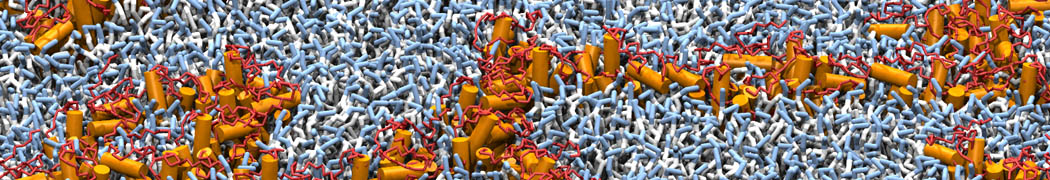
CG bonds/constraints and elastic networks
When a CG structure/trajectory is opened with VMD, the program builds a network of bonds using a distance criteria and an atomistic library of possible bond lengths (de ned by the namd force eld, developed by the same group); CG beads, linked with bonds with an average length of 0.35 nm, are not de fined through this automatic algorithm. VMD inevitably ends up displaying a cloud of dots, which are hard (impossible?) to properly visualize with non-bionic human eyes. A Tcl script which reads the bonds and constraints from the CG .itp/.tpr files, and rewrites the CG bond network is available on the Martini website.
First, make sure your system knows where to find the script:
source /wherever/cg_bonds.tcl
This script can now be used from the command line window of VMD as follows:
cg_bonds -top system.top -topoltype "elastic"
in case you have a .top available, but no gromacs. Alternatively, if gromacs is installed on the machine you are using, you may use a .tpr instead:
cg_bonds -gmx /wherever/gmxdump -tpr dyn.tpr -net "elastic" -cutoff 12.0 -color "orange"
-mat "AOChalky" -res 12 -rad 0.1
The last line will draw the ElNeDyn network with the options (cuto ff, color, material, resolution and radius) speci ed by extracting the bonds from the dyn.tpr file (that's where the gmxdump comes in). Note that you must specify a my gromacs version compatible with the dyn.tpr file.
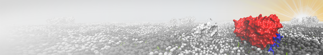
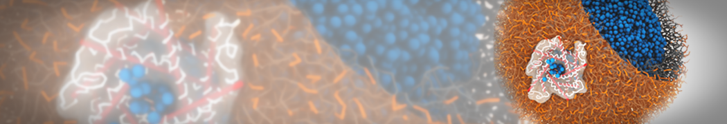
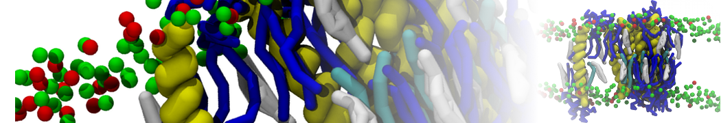
Visualization of secondary structure
After being able to draw bonds and constraints de ned by the CG force eld, the next step is to see protein secondary structure. We are currently developing a graphical script drawing vmd cartoon-like representation. This set of routines is still under development, and needs to be improved. . . by your feedback?
Two main routines are provided by the cg_secondary_structure.tcl script: cg_helix and cg_sheet.
Use these two commands in the same fashion:
cg_whatever {list of terminig} [-graphical options]
Or, in an example:
cg_helix {{5 48} {120 146}} -hlxmethod "cylinder" -hlxcolor "red" -hlxrad 2.5
which will draw two helices, from residue labeled as 5 to residue labeled as 48 and from residue labeled as 120 to residue labeled as 146, as red cylinder of radius 0.25 nm. Check the help shown when the script is sourced or the website for an exhaustive list of options and default values. To defi ne the list of termini, two options are implemented: i) providing the list by yourself (like in the example shown above), ii) reading/parsing a file generated by do_dssp. In the second case, you don't need to provide any termini, but the list of termini still needs to be written in the command line as an empty list: {}.
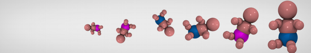
Please keep in mind that, due to the restricted amount of structural information carried on by a CG structure, the beauty and exactitude of these graphical representations are limited. . .