General Purpose Coarse-Grained Force Field

This is a brief tutorial on how to set up a simulation of a double stranded RNA molecule with the recent Martini force field parameters. Since RNA is very similar to DNA from the chemical point of view, the Martini RNA parameters are highly based on the DNA model. This also allows to have full compatibility with the DNA model and the other existing models in the Martini universe.

 

To make this tutorial more general, you should download the latest Martini DNA and RNA release from here. It includes the itp files for both molecules as well as a modified martinize script to coarse grain nucleic acids. As Martini DNA, Martini RNA can be used to model both single-stranded as well as double-stranded RNA. It also provides two separate elastic networks: a soft model has a cutoff of 1.2 nm and a force constant of 13 kJ mol^-1 nm^-2 and the stiff model has a cutoff of 1.0 nm and a 500 kJ mol^-1 nm^-2 force constant.

 

This tutorial will show only an example of creating a dsRNA topology using the stiff elastic network but a dsRNA topology with soft network or a ssRNA topology without elastic network can be created using the same procedure. For dsRNA structures the stiff elastic network is a good starting point for seeing how your system behaves in a CG simulation. There are also options for creating elastic networks for more complicated DNA structure; martinize-dna options all-stiff and all-soft are meant to be starting points for creating topologies for such structures but they are beyond the scope of this tutorial. The package includes a README file that should have sufficient instructions for creating the other types of RNA (and DNA) topologies after you have finished this tutorial.

 

1. Unpack the tutorial files you downloaded (it expands to na-tutorials).

 

 

2. Go to the folder na-tutorials/rna-tutorial/dsRNA-setup. Martinize works now also for RNA molecules. As for DNA, martinize-nucleotide.py for RNA works best with cleaned up .gro files so you should first remove other atoms from the .pdb file and convert it to a .gro file. You will find the .pdb file for the 1RNA pdb code. NOTE that a download from the PDB website can give you a file called 1rna.pdb. The file 1RNA.pdb (NOTE CAPIIALS) is provided in the archive, so you do not need to download.

 

 

3. Next we can use the script martinize-nucleotide.py (supplied for you in the current directory) to create a Martini RNA topology for 1RNA. 

 

 

 

 

 

 

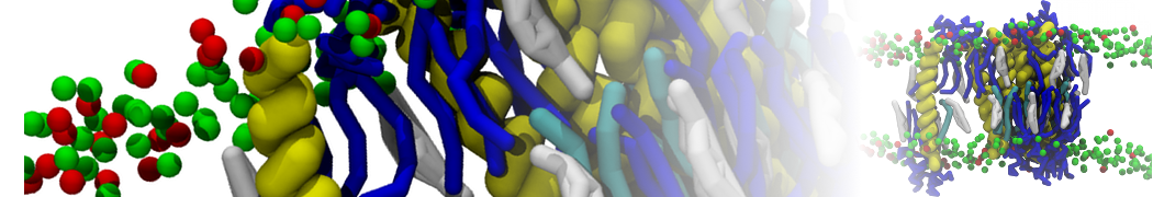
4. You can now visualize the mapping of the 1RNA molecule by opening both the atomistic and coarse-grained structures in VMD. (The visualization is clearer if you show the CG structure as small VDW spheres.)

 

 

5. Next you need to create a simulation box for the RNA molecule and solvate it as well as add counterions. You will find a pre-equilibrated coarse-grained water box in the downloaded folder. You can also download it from here.

 

 

You can replace water with ions in .top file without using genion at the same time as we add waters there. Note: the next line assumes that exactly 1226 water beads were added to the DNA by the genbox tool; the first 1100 added beads are designated as normal water beads, the next 100 beads are designated as anti-freeze water beads, and the final 26 beads are designated as sodium ions.  

 

 

6. Use the em.mdp provided in the directory to run an energy minimization (integrator = steep, nsteps = 100).

 

 

7. Next, you can run a short equilibration of 1 ns. Note, a smaller time step might be needed for initial equilibration (10 fs). 

 

 

8. Now you are ready to start your first RNA simulation. Use the mdrun.mdp file to produce a longer simulation. This time we will be running a 10 ns production run. Note that with the elastic network the domain cell size needs to be kept fairly large (option -rdd 2.0).

 

 

9. You can visualize the movements of the RNA, ions and waters using VMD while your simulation is still running (you will need to open a new terminal). Note that bonds in Martini are longer than bonds normally shown in VMD. Please consult the VMD tutorial to get better visualization.  It may be advisable to convert your trajectory so that molecules are not split over the periodic boundaries (using gmx trjconv -pbc whole) before viewing. It needs a bit more trickery to ensure that both RNA strands are shown close to each other, see the description in the protein tutorial.